PyTorch, torchvisionで提供されている学習済みモデル（訓練済みモデル）を用いて画像分類を行う方法について、以下の内容を説明する。

• 学習済みモデルの生成
• 画像の前処理
• 画像分類（推論）の実行

本記事におけるPyTorchのバージョンは以下の通り。バージョンによって仕様が異なる場合もあるので注意。

import torch
from torchvision import models, transforms

from PIL import Image

import json

print(torch.__version__)
# 1.7.1

コード全体は以下。

• pytorch-examples/image_classification_vgg16.ipynb - nkmk/pytorch-examples

学習済みモデルの生成

ここではtorchvision.modelsで提供されている画像分類のモデルVGG16を用いる。

vgg16 = models.vgg16(pretrained=True)

pretrained=Trueとすると、ImageNet（1000クラスの画像）で学習されたモデルが生成される。

torchvision.modelsでは、画像分類のモデルとしてVGGのほかにResNetやDenseNetなども提供されている。

• 関連記事: PyTorch Hub, torchvision.modelsで学習済みモデルをダウンロード・使用

画像分類のモデルであれば、以下で示す基本的な使い方は同じ。

画像の前処理

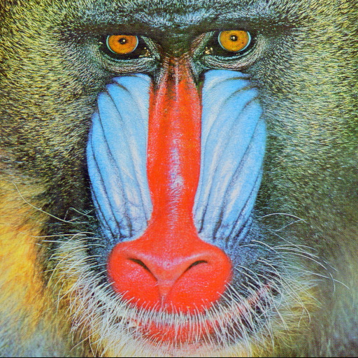
OpenCVにサンプルとして含まれているbaboon（ヒヒ）の画像を例とする。

• opencv/baboon.jpg at master · opencv/opencv

img_org = Image.open('../data/img/src/baboon.jpg')
print(img_org.size)
# (512, 512)

分類する画像は、モデルにあったサイズにリサイズし、学習（訓練）時と同じ前処理を行う必要がある。

torchvision.modelsで提供されている学習済みモデルの前処理は以下の通り。

All pre-trained models expect input images normalized in the same way, i.e. mini-batches of 3-channel RGB images of shape (3 x H x W), where H and W are expected to be at least 224. The images have to be loaded in to a range of [0, 1] and then normalized using mean = [0.485, 0.456, 0.406] and std = [0.229, 0.224, 0.225]. You can use the following transform to normalize: torchvision.models - Classification — Torchvision 0.8.1 documentation

torchvision.transformsを使うとこれらの前処理を簡単に実行できる。

• torchvision.transforms — Torchvision 0.8.1 documentation

transforms.Resize()とtransforms.CenterCrop()でリサイズ、transforms.ToTensor()でPIL.Imageからtorch.Tensorへの変換、transforms.Normalize()で正規化を行う。

それらの処理をtransforms.Compose()でまとめて実行する。

preprocess = transforms.Compose([
    transforms.Resize(224),
    transforms.CenterCrop(224),
    transforms.ToTensor(),
    transforms.Normalize(
        mean=[0.485, 0.456, 0.406],
        std=[0.229, 0.224, 0.225]
    )
])

img = preprocess(img_org)
print(type(img))
# <class 'torch.Tensor'>

print(img.shape)
# torch.Size([3, 224, 224])

transforms.Resize()は短辺が引数の値になるようにリサイズし、transforms.CenterCrop()は画像の中心から辺が引数の値の正方形をクロップする。例の画像は正方形なのでtransforms.CenterCrop()は不要だが、長方形の画像にも対応できるようにしている。

PyTorchでは画像の次元の並びが(チャンネル（色）, 高さ, 幅)なので注意。transforms.ToTensor()を使えば正しく変換してくれる。

PyTorchではバッチ処理が基本なので、1枚の画像の場合も先頭に次元を追加する必要がある。

img_batch = img[None]
print(img_batch.shape)
# torch.Size([1, 3, 224, 224])

Noneで次元を追加するのはNumPy配列numpy.ndarrayと同じ考え方。

• 関連記事: NumPy配列ndarrayに次元を追加するnp.newaxis, np.expand_dims()

torch.unsqueeze()を使う方法もある。

• torch.unsqueeze() — PyTorch 1.7.1 documentation

print(torch.unsqueeze(img, 0).shape)
# torch.Size([1, 3, 224, 224])

画像分類（推論）の実行

モデルで推論（予測）を行う前に、eval()で推論モードにセットする。

• torch.nn.Module.eval() — PyTorch 1.7.1 documentation

vgg16.eval()

DropoutやBatch Normalizationなどの訓練時と推論時で振る舞いが異なるレイヤーがある場合はeval()を実行しておかないと正しい結果にならないので注意。

なお、訓練モードにセットするのはtrain()。

• torch.nn.Module.train() — PyTorch 1.7.1 documentation

モデルに画像のテンソルを渡して、推論を実行する。

結果もテンソルtorch.Tensor。1枚の画像の1000クラス分類なので、形状は(1, 1000)となる

• 関連記事: PyTorchのTensorの次元数、形状、要素数を取得: dim(), size(), numel()

result = vgg16(img_batch)
print(type(result))
# <class 'torch.Tensor'>

print(result.shape)
# torch.Size([1, 1000])

何番目のクラスの値が最大か（＝どのクラスである可能性が一番高いか）をtorch.argmax()で取得。0次元のtorch.Tensorが返される。

• torch.argmax — PyTorch 1.7.1 documentation

idx = torch.argmax(result[0])
print(idx)
# tensor(372)

print(idx.ndim)
# 0

ImageNetのクラスのデータは色々なところで公開されているが、ここではKerasで使われているものを使う。

• keras/imagenet_utils.py at master · keras-team/keras
• imagenet_class_index.json

以下のように、Python標準ライブラリのjsonモジュールを用いて、'0'から'999'までの文字列をキーとする辞書dictとしてデータを読み込む。

• 関連記事: PythonでJSONファイル・文字列の読み込み・書き込み

with open('../data/imagenet_class_index.json') as f:
    labels = json.load(f)

print(type(labels))
# <class 'dict'>

print(len(labels))
# 1000

print(labels['0'])
# ['n01440764', 'tench']

print(labels['999'])
# ['n15075141', 'toilet_tissue']

0次元のtorch.Tensorからitem()で値を取り出しstr()で文字列に変換してキーとする。

• 関連記事: PyTorchのTensorの要素の値を取得: item()

print(labels[str(idx.item())])
# ['n02486410', 'baboon']

baboonと正しく分類できていることが確認できた。

分類の確率を取得したい場合は、結果に対してソフトマックス関数を使う。合計が1となるように変換される。

• torch.nn.functional.softmax() — PyTorch 1.7.1 documentation

probabilities = torch.nn.functional.softmax(result, dim=1)[0]
print(probabilities.shape)
# torch.Size([1000])

print(probabilities.sum())
# tensor(1.0000, grad_fn=<SumBackward0>)

baboonの確率は以下の通り。0次元の整数intのtorch.Tensorはそのままインデックスとして指定可能。もちろんitem()を使っても構わない。

print(probabilities[idx])
# tensor(0.5274, grad_fn=<SelectBackward>)

print(probabilities[idx.item()])
# tensor(0.5274, grad_fn=<SelectBackward>)

上位のクラスとその確率を取得したい場合は、torch.sort()を用いる。

• torch.sort() — PyTorch 1.7.1 documentation

torch.sort()はソートされた値とインデックスを返す。ここでは値は使用しないので_に代入している。

• 関連記事: Pythonでタプルやリストをアンパック（複数の変数に展開して代入）

_, indices = torch.sort(result[0], descending=True)
print(indices.shape)
# torch.Size([1000])

for idx in indices[:5]:
    print(labels[str(idx.item())][1], ':', probabilities[idx].item())
# baboon : 0.5274456143379211
# guenon : 0.2361937314271927
# patas : 0.08894255757331848
# vulture : 0.05698851868510246
# crane : 0.015375789254903793